14. Impact of Effective Lens Position on Refraction

The quality of predicting the actual position of the implant (effective lens position, ELP) is what distinguishes modern formulas for intraocular lens (IOL) power calculation. This prediction is made using methods unique to these formulas, some of which, like the PEARL DGS formula, benefit from the contribution of artificial intelligence (AI).

Is it possible to quantify the impact of a variation in the effective lens position on the refraction of the pseudophakic eye?

Does it depend on the power of the implant? On the power of the cornea? And if so, to what extent?

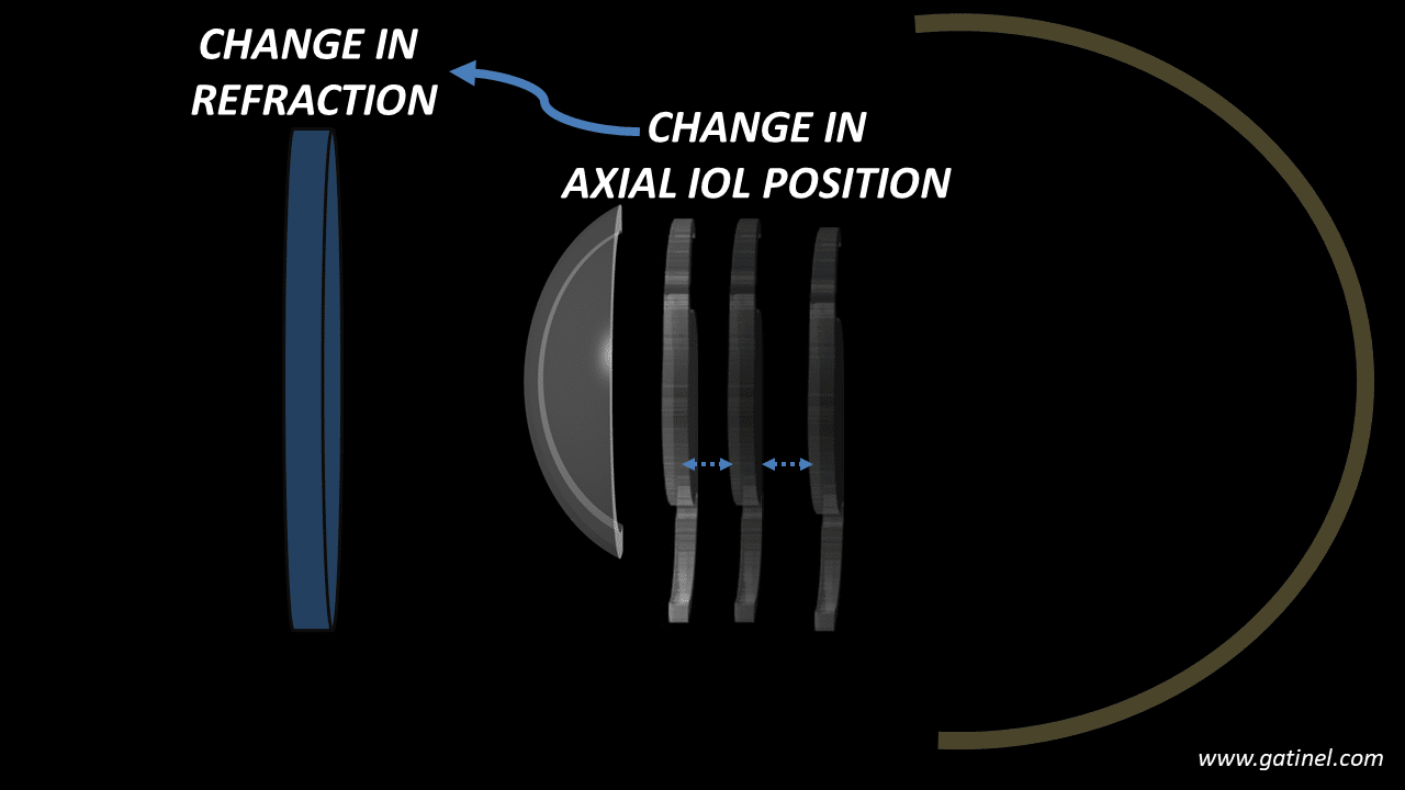
How does a change in the Effective Lens Position (ELP) within the pseudophakic eye affect its refraction?

This page aims to answer these questions.

Understanding the impact of the Intraocular Lens (IOL) position on the refraction of the pseudophakic eye is crucial for grasping the challenges associated with optimizing the constants in IOL power calculation formulas. These issues will be discussed at the end of this page.

1. Definitions of Effective Lens Position (ELP):

It is essential to differentiate between models of pseudophakic eyes composed of thin lenses and those that incorporate the thickness and respective powers of the anterior and posterior corneal surfaces. The fact that first-generation formulas were thin-lens formulas led to certain inaccuracies, necessitating the need for optimization through the adjustment of constant values. The effect of these adjustments is to vary the ELP (Effective Lens Position).

-Thin Lens Eye Models:

In this type of system, where the cornea and lens are considered to have negligible thickness, the effective lens position is simply the distance separating these two elements.
Accounting for the anatomical distance between the cornea and the lens can be conducted in various ways; typically, the distance between the corneal vertex and the anterior surface of the implant is chosen. The thickness of these elements is disregarded, which allows for the treatment of a relatively simple system. However, this results in a loss of precision, as the impact of the geometry of the cornea and the IOL is not negligible. Suppose a thick lens is considered a thin lens. In that case, it is not possible to take into account the effect of geometric variations of the surfaces of the constituent elements involved (anterior and posterior surfaces of the cornea and the IOL and the distances that separate them).

-Thick Lens Models:

This type of model allows for the consideration of the thickness of the cornea and the implant, as well as their respective anterior and posterior curvatures. The principal planes are theoretical constructs that allow for the simplification of thick systems into thin systems while preserving their characteristics. The power of an equivalent thin system is calculated based on the powers of the front and back surfaces and the thickness of the element it replaces. Its position is transferred to the object or image’s principal plane depending on its location with respect to the incident rays.

In this model type, it is thus convenient to refer to the principal planes of the thick lenses used (cornea and lens). The ELP is the distance separating the cornea’s principal image plane from the implant’s principal object plane. The position of these planes depends on the respective curvature radii of the anterior and posterior surfaces of the considered element.

The cornea’s principal planes are always located very close to the anterior corneal surface, whereas the principal planes of IOLs greatly vary with their optical design. Thin-lens-based formulas would be as accurate as thick-lens formulas only if the IOLs’ principal planes were always in the same position relative to the optics.

It is possible to consider that an equivalent thin lens system can replace a thick lens system provided that:

-The power of each lens has been calculated based on the power of each constitutive surface and the distance separating them. In this context, the optical power of the cornea and the IOL must be calculated based on their thickness and the curvature of their anterior and posterior surfaces (these calculations are detailed for the cornea and the IOL).
-These equivalent thin lenses are placed respectively at the principal image plane for the cornea and the principal object plane for the IOL.

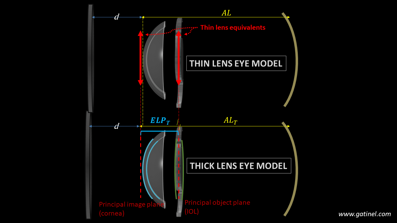
Representation of the equivalent thin and thick lens pseudophakic eye models. The values of the ELP and AL must be adapted using the location of the principal planes of the cornea and IOL for a thin lens eye model to replace an equivalent thick lens eye model.

Thus, in what follows, the Effective Lens Position refers to a distance separating the corneal and the IOL, whether obtained from a thin lens model or resulting from the transformation of a system composed of thick lenses (i.e., the distance between the aforementioned principal planes). In a primitive thin lens system, variations in the ELP (Effective Lens Position) are akin to a variation in the physical position of the lens. In a thick lens system, variations in the ELP can result from anatomical position changes and/ or optical design variations without any anatomical displacement of the implant’s optics relative to the cornea. Let us focus on this point.

-Anatomical vs optical variation in Effective Lens Position

It is important to understand that taking into account the geometry of the refractive elements implies that it is possible to induce variations in ELP linked to geometric/structural variations (e.g., distribution of power between the front and back surface of the IOL) without the anatomical/physical distance between the cornea and the IOL being modified. Variations in IOL style (modification of the power distribution between the front and back surfaces, i.e., changes in the Coddington factor) are likely to explain the refractive errors induced when changing the type of implant, assuming moreover that the position of the optic in the capsular bag is nevertheless unchanged. This is, of course, linked to the fact that the position of the principal planes of the IOL varies with the power distribution between the element’s surfaces. Unfortunately, this distribution (the optic design) is rarely disclosed by the IOL’s manufacturers.

Let’s consider an extreme case: that of two 22D implants; one is plano-convex (the back surface is responsible for the convergence of light rays), and the other is convex-plane (the front surface carries the entire optical power of the implant). For the same anatomical distance separating the cornea from the front face of these implants, the ocular refraction will be more convex (or less concave) with the plano-convex geometry implant. Its principal object plane being closer to its posterior surface, the value of the ELP (Effective Lens Position) in a thick lens eye model will be greater than for the convex-plano implant.

It is, therefore, essential to understand that variations in the ELP (Effective Lens Position) include both the physical movements of an implant and its optical design variations.

Impact of IOL design on ELP and refraction of the pseudophakic eye. The anatomical location is identical for the two IOLs. Still, the position of its principal planes is more posterior for the IOL, which has most of its optical power distributed by its posterior surface (bottom). As a result, it is as if this lens were further away from the cornea. The ELP being longer, the refraction of this eye is less concave (more convex).

We have investigated the consequences of the variations of lens design on the accuracy and precision of IOL power formulas (causing deviations in ELP values), using both theoretical and disclosed IOL designs (read here)

2. Impact of ELP variations on Refraction:

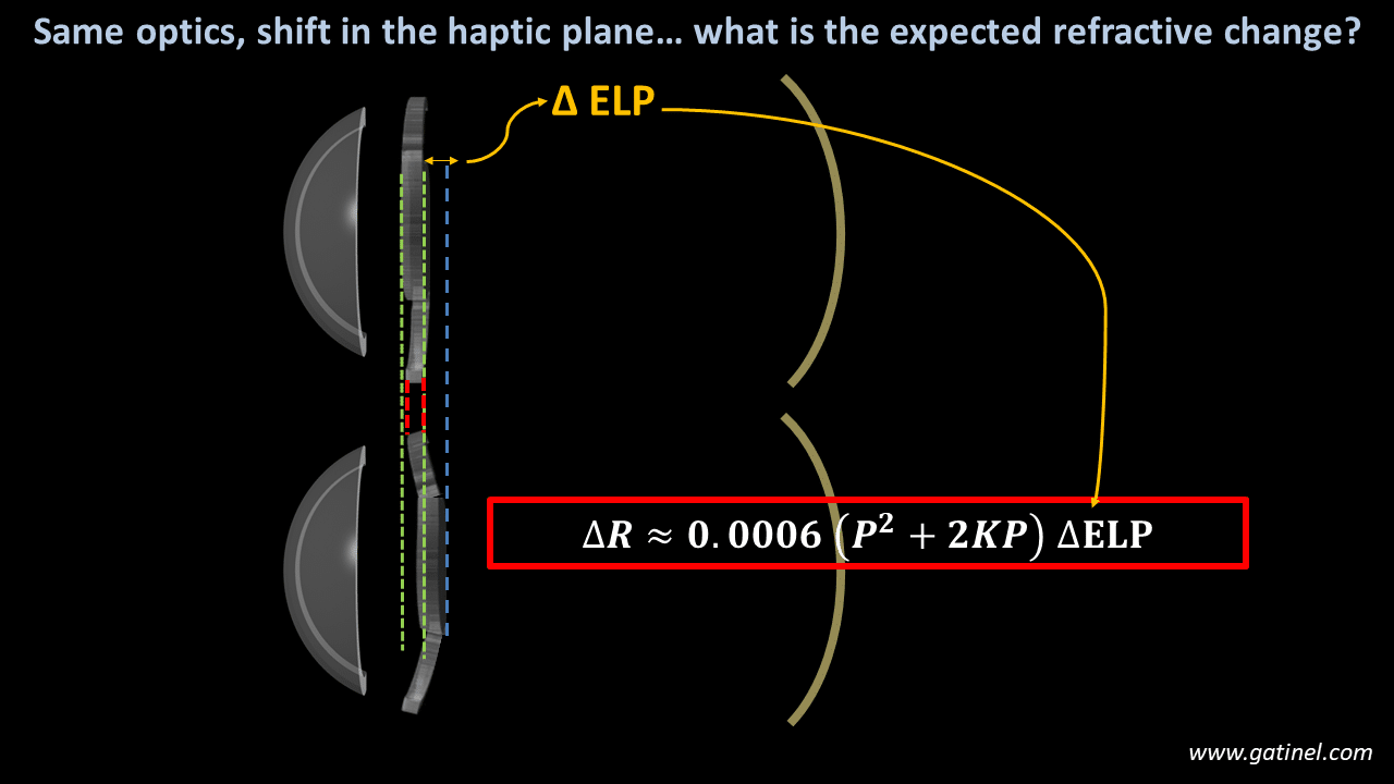
In previous work, we proposed a formula to approximate the impact on refraction of an axial displacement of an implant (anatomical and/or optical) with power P placed behind a cornea with power K.

This relationship is as follows:

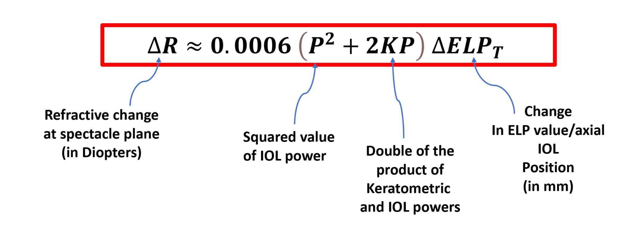
The analytical formula relating the change in ocular refraction with the change in ELP of the IOL.

This equation demonstrates that the relationship between refractive change (ΔR) and implant displacement (change in ELP, ΔELPT) is linear, given a constant corneal power and a fixed IOL power.

Right away, we can see the significance of the implant’s power within this ELPvsRefraction formula: its square and its product with the corneal power are involved in the calculation.

This relationship highlights that the impact of a variation in the implant’s position is substantially the same regardless of the initial value of the effective lens position.

NB: The (lengthy) derivation of this formula is available in an Appendix.

-Examples of calculation

What is the expected change in refraction caused by a shift of 0.1 mm in the ELP in a pseudophakic eye with IOL power P= 22D and keratometric power K=43D?

The answer is ΔR=0.0006 x (22^2 + 2 x 22 x43) x 0.1 = 0.127 D

Suppose that the IOL power would be 5D: for the same IOL shift,  ΔR=0.0006 x (5^2 + 2 x 5 x43) x 0.1 = 0.027 D, which is quite less.

Conversely, repeat the calculation with IOL P= 35 D, ΔR=0.0006 x (35^2 + 2 x « 5 x43) x 0.1 = 0.254 D, which is much more.

Considering the anterior chamber depth at 3 mm and the lens thickness of around 5 mm, compared to the implant thickness of about 1 mm, uncertainty in the implant’s position on the order of a millimeter is plausible. The primary quality of a good power calculation formula is its ability to accurately predict the implant’s position (ELP). The geometry of most lenses (anterior vs. posterior power ratio) is not disclosed by manufacturers, which complicates the prediction task.

-Influence of the IOL power:

This graph shows the impact of the IOL power on the expected change in ocular refraction for a 1 mm variation in ELP.

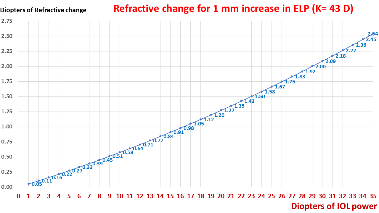
This graph displays an exponential relationship between the change in refraction and the IOL power when the ELP is altered by 1 mm.

For the same change in position, the refractive change doubles for a 29-D implant compared to a 17-D implant.

-Influence of the Cornea:

This graph shows the impact of the IOL power on the expected change in ocular refraction for a 1 mm variation in ELP.

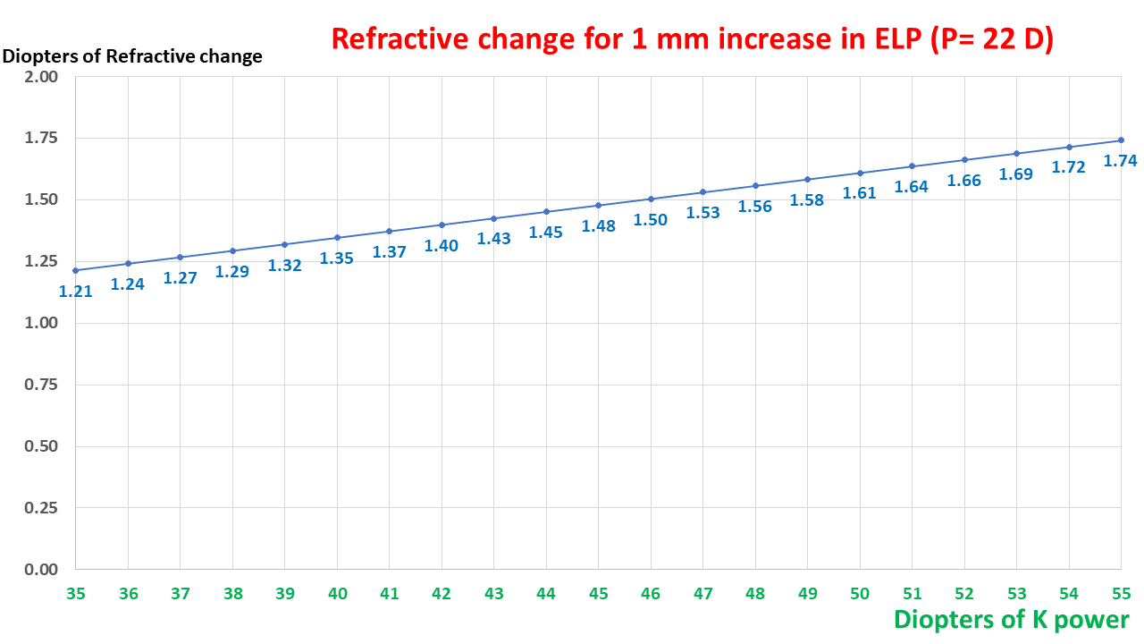
Expected change in refraction for an increase of 1 mm in ELP as a function of keratometric power. The relationship is linear.

As suggested by the ELPvsRefraction formula, the impact of keratometry is linear and smaller than that of the IOL power.

3. Applications

Being able to accurately estimate the impact of the variations of ELP  on the refraction of a pseudophakic eye is useful in many clinical circumstances:

-Anticipating the impact of implant design variations.

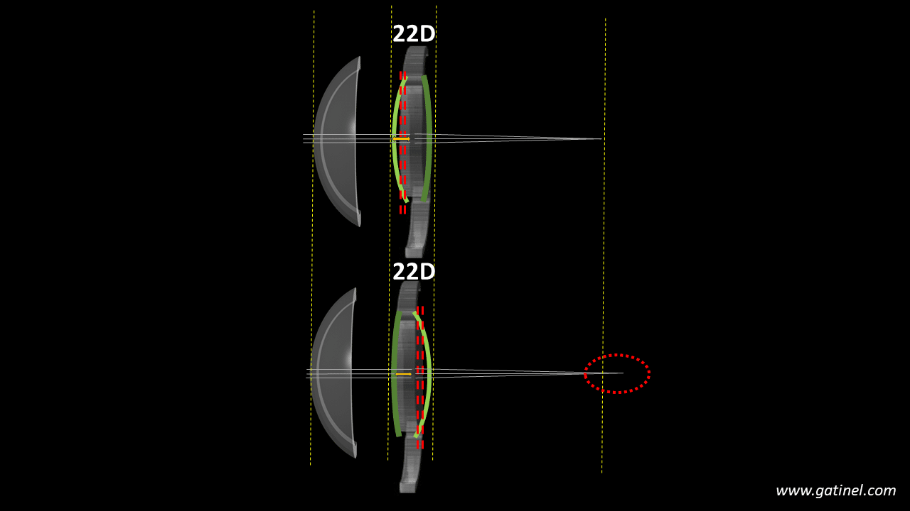
-Optic design variations :

If the values of the front and back radii of curvature, the refractive index, and the thickness of an implant are known, it is possible to calculate the position of its principal planes. Any design variation (at constant power) shifts the principal object plane. The value of this shift is equivalent to a variation in the ELP (Effective Lens Position). Due to variations in design among available IOLs, it’s necessary to « correct » implant calculation formulas by adjusting their optimization constants. Our analytical formula allows for estimating the expected refractive variation caused by the design change.

-Haptics design variations

A modification of the location of the haptic plane/angle relative to the optics is equivalent to an anatomical displacement of the implant, hence a variation of ELP.

Assuming an isolated change in the haptic angle of a specific IOL model, which induces an identical shift of the optic plane with the range of IOL regardless of their respective power. The refractive impact of this variation can be calculated using the formula: this impact greatly depends on the power of the considered implant.

In both scenarios, one can predict the refractive outcome in a pseudophakic eye, considering the powers of the IOL and cornea, provided that the lens displacement is accurately measured. This approach enhances the precision in forecasting postoperative refraction by taking into account the lens’s exact position within the eye.

-Analyzing refractive surprises

Having an equation that relates the position of an implant to ocular refraction allows us to assess the impact of an error in predicting the Effective Lens Position (ELP) on the generation of refractive surprises. It is sufficient to measure any difference between the expected and actual position of the IOL and calculate the refractive impact of this difference. In principle, low-power implants are resilient to the actual ELP because the variations induced by their axial position changes are very small.
The position of the implant can be measured using anterior segment OCT imaging. The ELP (Effective Lens Position) value can also be calculated retrospectively, providing a more accurate understanding of the implant’s location, which is crucial for investigating the refractive impact of the IOL on the ocular refraction.

-Optimization of IOL power formulas

Optimizing formulas through a constant adjustment relies precisely on an expected position offset of the IOLs. This variation in position aims to minimize the average prediction error of an implant calculation formula. The exponential relationship between refractive variation and implant power emphasizes that, on a given dataset, formula optimization will mainly occur with high-power IOLs.

The ELPvsRefraction formula enables the conception of a simplified method for optimizing IOL power formulas.

This area is important but often misunderstood due to being rife with approximations and erroneous assumptions. We will take advantage of what we have learned to delve deeper into this matter and unravel the mystery of the impact of constants in the field of IOL power calculation in the next section.

4. Enhancing precision with lens constant optimization:

In this section, we will expose the knowledge required to understand a topic frequently subject to misunderstandings, and that can lead to confusion as its complexity extends beyond initial appearances.

-Preliminary remarks

-Any formula utilizing an optical calculation kernel must first predict the actual position of the implant (the effective lens position) in order to accurately determine the IOL power required for the implanted eye to achieve the desired postoperative refraction.

-The prediction of the effective lens position is made based on the biometric characteristics of the eye being operated on.

-In the context of a post-operative analysis, the IOL power formula is evaluated by comparing the postoperative refraction achieved to the refraction predicted by the formula with the considered IOL model of a given power in a given eye. (For reasons not elaborated here, the optimization is based on the quality of a postoperative refraction prediction with a given implant rather than the quality of a power prediction to be placed to achieve actual postoperative refraction. In other words, the accuracy of the formula is not determined by comparing the predicted IOL power needed to achieve postoperative refraction with the actual power of the implanted IOL).

-The difference between the refraction achieved, and that predicted by the formula for an implant of a given power in a given eye corresponds to the refractive prediction error in that given eye. (As underlined above, this is significantly different from clinical practice, where a formula is used to predict the power of an implant to be placed in order to achieve target refraction; nevertheless, achieving a zero prediction error via constant adjustment will allow the formula to predict better the powers of IOls intended to induce target refractions in future operated eyes).

-What is a lens constant?

Constants are numerical values that can be incremented to vary the predicted position of a specific IOL model. Most formulas use only one such constant (they are « single-optimized); some, like the Haigis formula, can use three, one of which is equivalent to that of a « single-optimized » formula.

The Haigis formula predicts the Effective Lens Position (ELP) for a given eye using a multiple linear regression equation that includes axial length (AL) and preoperative anatomical anterior chamber depth (ACD), expressed in mm.

ELP=a0 + a1*ACD + a2*AL

The coefficients a0, a1, and a2 in this formula are specific to each implant model. When adjusting the a0 constant in the Haigis formula, the increment applied is the same for all eyes, meaning this adjustment uniformly affects the calculation of the Effective Lens Position (ELP) across different patients, regardless of their individual eye characteristics. This universal application helps standardize the adjustment process for ELP prediction in the Haigis formula.

-Refractive impact of the lens constant variation:

When the constant is modified, the initially predicted effective lens position by the formula for each eye in the set is changed by the same value. However, the refraction predicted by the formula varies according to the power of each implant, in light of what we have studied earlier. The refractive change increases exponentially with the power of the IOL, linearly with the corneal power.

-Initial lens constant determination:

For a given IOL power formula, the value of the constant is initially adjusted based on retrospectively studied data concerning the accuracy of the prediction regarding a specific IOL model.

The online platform IOL Con provides ophthalmologists with specifications and optimized constants for lenses of all major manufacturers.

However, a surgeon may find that they do not achieve an average prediction error of zero with the recommended constant value due to variations related to the profile of the operated eyes, variations in their biometric measurements, etc.

In such cases, it might be advisable to optimize the value of the constant to nullify the mean prediction error.

– Optimization of the IOL constant

It is crucial to fully understand the reasoning and method used for optimizing an implant calculation formula via constant fine tuning. To do this, it is advisable to read the following very carefully, especially if you are not yet familiar with this type of approach:

-To optimize a formula for a specific IOL model, a documented dataset is needed. The dataset includes preoperative biometric data of operated eyes and the postoperative refraction obtained for each eye that received the same IOL model, the power of which is also known.

-In a single-operated eye, the difference between the achieved refraction after IOL implantation and the predicted refraction equals the prediction error (be careful not to confuse the refractive prediction error with the postoperative refraction). For instance, if a formula predicts that for a given eye and a 22D IOL, the refraction should be -1D, but in practice, the achieved refraction was -1.50 D, the refractive prediction error would be -1.50 – (-1) = -0.50 D.

-In clinical practice, the global average prediction error made by the formula is the average of this error across all operated eyes of a studied documented dataset.

-We then have a documented dataset where we know the power of the IOLs that were placed in each eye and the preoperative biometry and refractive prediction error for each eye. If the average of these errors (the mean prediction error) is not zero, it is desirable to optimize the formula by adjusting the optimization constant.

-To achieve a zero global average error, one can shift the predicted position of the implants by a constant increment. As we know, this modifies the predicted refraction specific to each eye of the dataset. This implies that a non-zero average prediction error is related to a systematic error in predicting the position of implants (in practice, this is rarely the sole cause).

-To nullify the average error, it is sufficient to determine the value of the adjustment that induces a zero average mean prediction error. Several methods are possible to determine this value, and we have proposed a simplified method to achieve this goal.

-Our predictive ELPvsRefraction formula highlights a paradoxical effect of the classic optimization by constant adjustment. The compensation for this systematic bias is achieved via a constant positional increment by a variation in the refractive prediction of the formulas that are not constant across operated eyes. Short eyes, for which a significant power is required, contribute more to the necessary refractive variation for zeroing than long eyes.

-Exploring the effect of changes in the IOL constant (such as the A-constant) on the refractive outcome.

Changing the constant of a formula, such as the Hoffer  (pACD), Holladay (SF), and Haigis (a0) formulas, amounts to varying the value of the ELP (Effective Lens Position) predicted by a formula by a constant increment (in mm). Hence, one can replace ΔELPT with the variation in any of these constants to estimate the refractive change incurred.

The positional constant of the SRK T formula is called the ACD-const. It is related to the A constant through a regression formula (the relationships between these elements are detailed on this page). A change of one unit in the A-constant results in a variation of 0.62467 mm in the predicted position of the IOL (i.e., the effective lens position).

Therefore, the ELPvsRefraction equation can be rewritten to adapt to a variation in the A-constant:

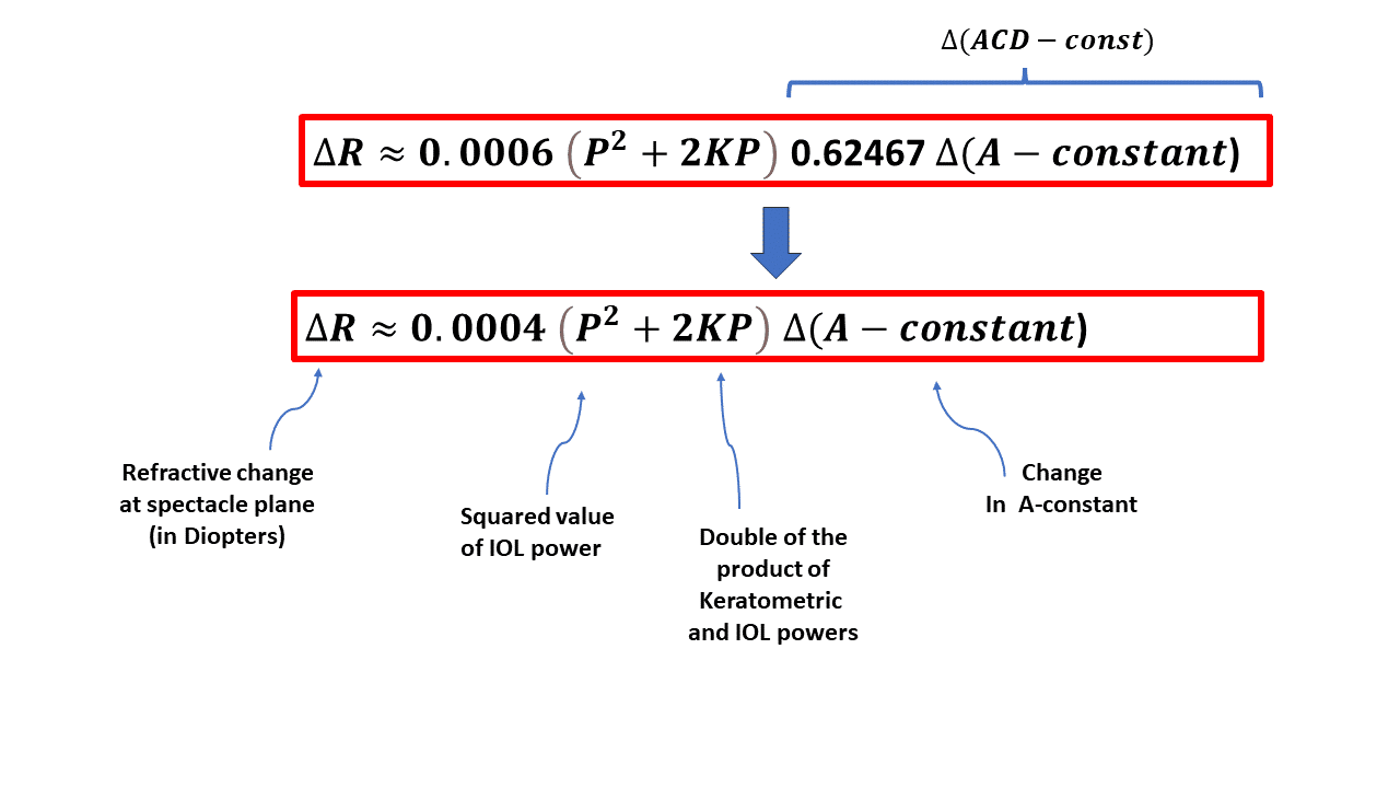
Approximation of the refractive impact of a variation in the A-constant.

When the SRK-T formula predicts certain refraction for a 22D implant and a 44D cornea and a certain A-constant, a variation of 1 unit in that A constant would result in a variation of 0.0004 (22^2 + 2*22*2*22)=0.002*22^2 = 0.968 D of the predicted refraction, which is practically 1D, this « coincidence » (not entirely fortuitous) explains the frequent confusion between the A-constant of the SRK formula (which has a direct impact on the power of an implant, hence on the ocular refraction) and that of the SRK-T formula. For low or high-power IOLs, this equivalency is lost.

-Examples

A power calculation report for an IOL includes the biometric information necessary for the predictive calculation of the implant’s power. This power aims to achieve the set refractive target (emmetropia or mild myopia). The prediction of the ELP (Effective Lens Position) is necessary to calculate the power of the IOL; it is not disclosed in the output of the biometer. What is displayed is the adjustment constant that comes into play in the calculation. It is chosen based on the implant model and has been previously adjusted based on the retrospective study of documented data as previously described.

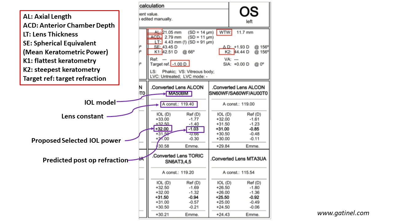
Biometry report figuring data used for IOL power calculation and the proposed IOL power.

Let’s test our ELPvsRefraction formula to verify if the refractive change it predicts matches what is displayed by the biometry report:

-SRK-T formula

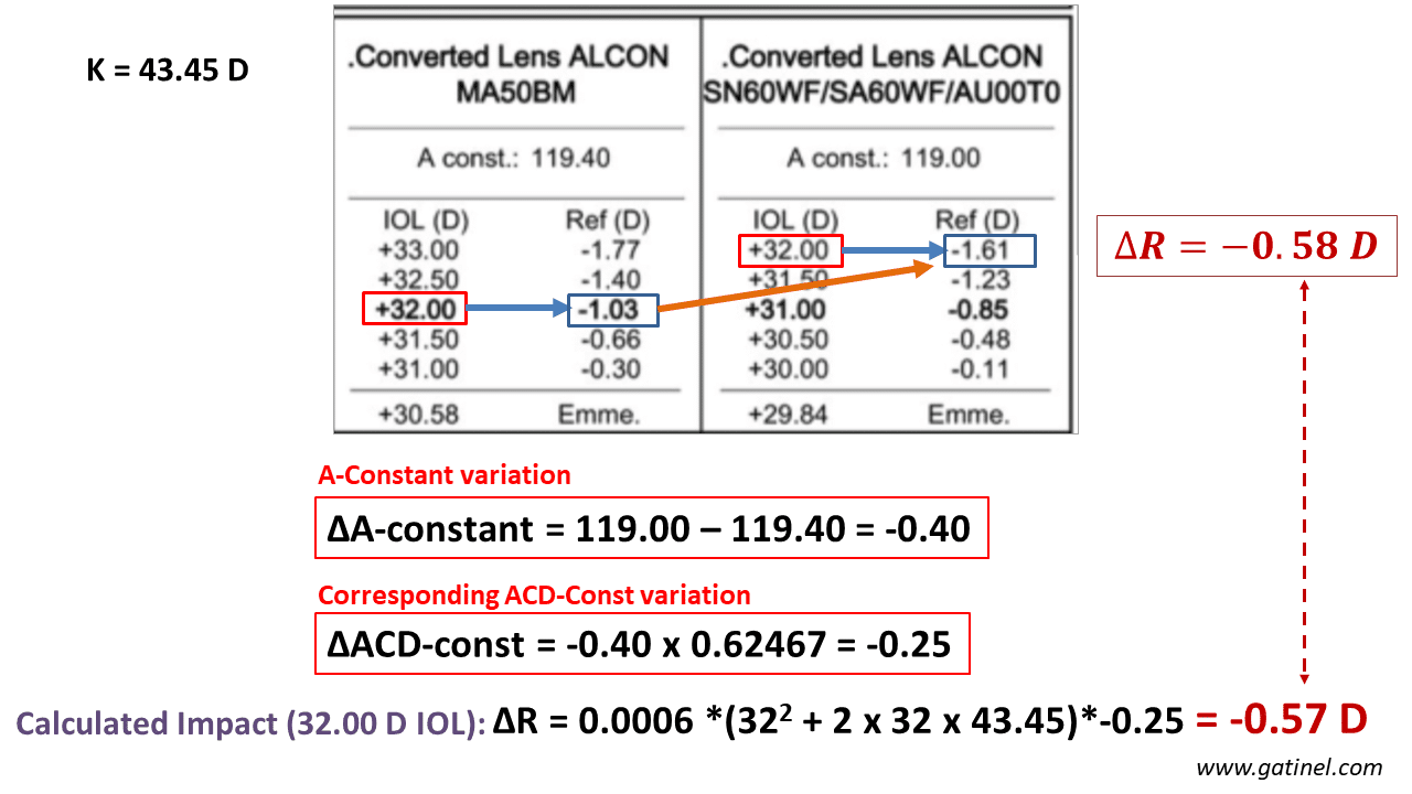
Comparison between the refractive change predicted by the implant calculation formula and our ELPvsRefraction formula for a variation of A-constant related to a change in IOL type. The calculation is performed for a 32D power. The difference is negligible.

-Haigis formula

Another example is displayed: the formula used is Haigis, and the adjustment constant is a0:

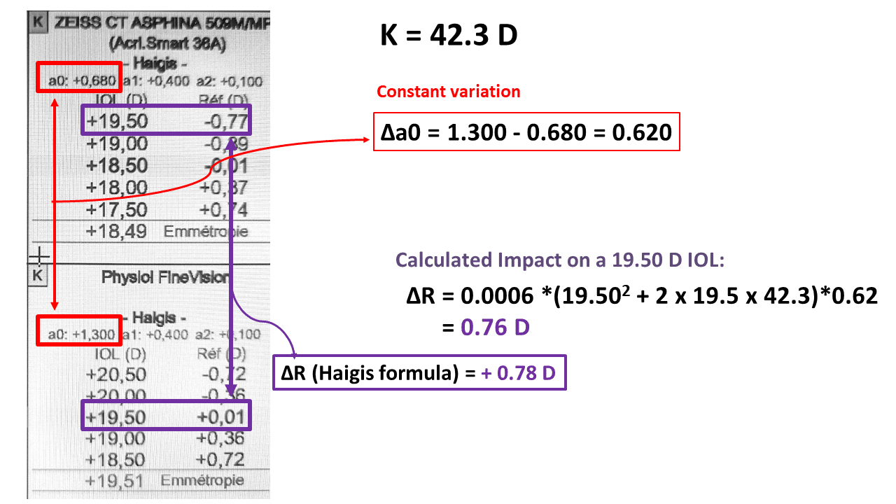
Haigis formula: impact of a0 constant change on postoperative predicted refraction (tested IOL power: 19.50 D).

In this example, the constants a1 and a2, which remain unchanged, are related to the axial length and the preoperative anatomical depth of the anterior chamber. They contribute to the prediction of the ELP; however, only variations in a0 affect all eyes by the same increment for ELP calculation, indicating a0’s unique role in adjusting the formula to account for differences in IOL style. Our ELPvsRefraction equation provides a good estimation of the refractive change incurred by the variation in ao (0.76 vs 0.78 D).

Conclusion

The effective lens position (ELP) exerts a strong influence on refraction post-intraocular lens (IOL) implantation, emphasizing the need for precision in IOL power calculations. These findings underscore the complexity of achieving accurate refractive outcomes due to anatomical and optical variations affecting ELP. These findings highlight the importance of accounting for individual anatomical and optical variations in ELP and the need for precise adjustment of lens constants in calculation formulas to improve the predictability of postoperative refraction.

Related content: Optimizing IOL power formulas.