WAVEFRONT SENSING CAN MAKE SENSE !
An introduction to help you familiarize yourself with the basics of WAVEFRONT ANALYSIS
Target Audience : Clinicians and Ophthalmic Practitioners
INTRODUCTION
Since the emergence of wavefront sensing technology, there has been a resurgence of interest in Optical Wavefront Analysis as a subset of Adaptive Optics (AO). Previously, we were happy to see a patient in clinic with 6/6 snellen visual acuity after correcting their spherocylindrical refractive error with glasses.Persistent visual symptoms, despite optimal spectacle correction, can now be qualified and quantified using wavefront analysis, which allows us to correlate specific types of aberrations with the visual complaints of the patient. This new technology has enabled us to develop Wavefront-Guided Refractive treatments, including LASIK, custom-fitted contact lenses, and Customized Intraocular lenses. Additionally, it has allowed us to acquire ultra-high-resolution imaging of the retina by compensating for aberrations. We are starting to aim for ‘super-normal’ vision (natural uncorrected VA of 20/15 or better) and really beginning to understand the optics related to visual performanceof the eye.
Now we know why Wavefront Sensing is pertinent to modern ophthalmic clinical practice. Here are the salient points about the technology in the form of answers to the questions below!
Light : Rays, Waves and Photons?What is a Wavefront?What is a Wavefront Aberration/Error?What are the types of Aberrometers? Focus: Shack-Hartmann wavefront sensorHow is the Wavefront Analysed? Focus: Zernike polynomialsRetina and Pupil plane Metrics Uncovered! Focus: PSF and RMS NEXT PAGE: Zernike polynomials EXPLAINED!
Optical simulator for Zernike aberrations
Some of these terms may seem esoteric to the unfamiliar clinician : hopefully this page will come to your rescue!
Light : Rays, Waves and Photons?
Light is a form of electromagnetic radiation. The human visible spectrum, which is the range of wavelengths visible to the human eye, sits between UV and Infrared, with wavelengths in the range of 380-750 nanometers. In the section below we invite the reader to move from the domain of geometric optics, where light propagates as ‘rays’; to the domain of wavefront optics, where light propagates as ‘waves’. We will not discuss the more complex and less relevant Quantum optics here, where light travels as ‘photons’. In fact, one can say that a ray is the path of a photon or the direction of a wave.First, let us consider a « perfect » optical system (top), and a « perfect » eye (bottom)
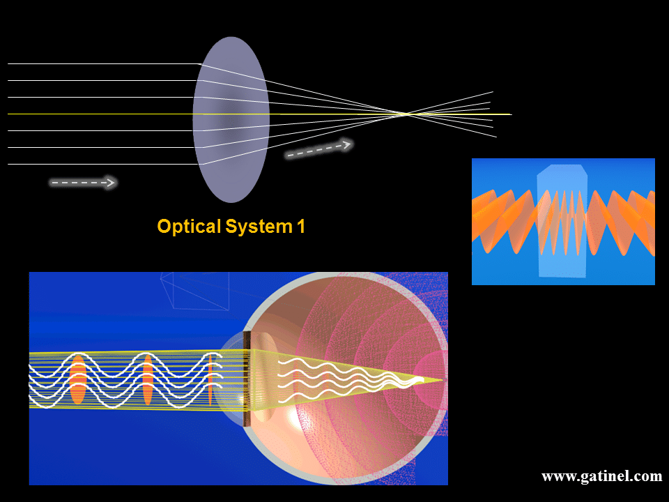
Light rays are, in fact, hypothetical representations of the assumed path of « light », which travels in a straight line through the emptiness of space. They can be refracted at each optical interface (the surface of a lens, the cornea, etc.), and a change in the direction of the path obeys the « law of refraction,» also known as « Snell-Descartes or Snell’s law ».
Light rays can also be imagined as the path taken by photons, light energy particles without mass. Photons can only be « seen » once they have interacted with some photosensitive membrane; they are of little help here.Finally, light rays can represent the direction in which “light waves” interfere in a constructive manner. Light waves represent the oscillation of the electromagnetic field. All this can be simplified, and the trajectory of the oscillation of the electromagnetic field represented as a longitudinal sine wave, where crests and troughs alternate regularly. The distance between two consecutive crests (or troughs) is the wavelength of the emitted light. Most natural light sources are polychromatic. In contrast, laser light is almost entirely (although not completely) monochromatic. Wavefront analysis is performed using infrared light, and the following discussion assumes a monochromatic source of light. Infrared light is invisible to the human eye but can travel through ocular media and to be reflected by the retina. These qualities make wavefront analysis possible and, at the same time, practical for the patient.
What is a wavefront?
A wavefront is an abstract construction that is formed by a surface joining the points of the same phase, at the same time, for a series of light waves (constructive interference), much like ripples on the surface of water when it’s raining. The previous figures depict the points all located at the top of the light waves’ crests. The light rays and wavefront are mutually perpendicular: light rays may be conceived as lines that define the local direction of the wavefront propagation.
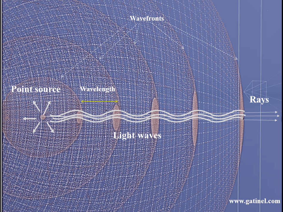
The shape of a wavefront can vary depending on the geometry of the source (point, linear, etc) and can be spherical, cylindrical, plane, concave or convex. As light travels from a star to the eye, the points that are « in phase » and which will be captured by the eye within its pupil are located on a flat disc, creating a plane wavefront. Light slows when travelling in a more « dense » transparent material, such as the corneal stroma. The higher the refractive index of the material, the slower the speed and the shorter the wavelength becomes.Due to the geometry of the eyeball, and the fact that light waves shorten (the speed or velocity of light is reduced) in the ocular media, the phase relations are modified: the convexity of the corneal dome and the variable thickness of the crystalline lens causes the peripheral light waves to be less delayed than the central ones. Peripheral waves travel slightly further in the air than central ones, which first hit the corneal apex, and are thus delayed relative to the peripheral waves. Light waves are guided toward a point where they can arrive in phase, where the oscillations will addup to increase the amplitude of the electromagnetic field oscillations. The intensity of light (energy) is proportional to the square of the amplitude of the oscillations E ∝ A2.Suppose that you could reverse the path of time, what would happen to the light waves emitted by a star? The light would travel back along the same rays, concentrically, and arrive in phase at the center of the star (where it was emitted « in phase » if the source is « coherent »). To form a bright image of a star, we need some of the emitted light waves to interfere constructively at a point and locate that point on a photosensitive membrane (such as a screen or the photoreceptor layer of the retina).
If the eye is a « perfect eye », then the location where the light waves interfere constructively after travelling through the anterior segment is at the fovea. In the vitreous cavity, the surface joining the points that are in phase would form an exact portion of a sphere centered on the fovea.
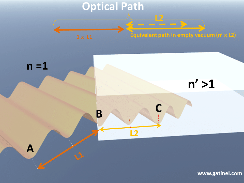
The optical path
From the star to the fovea, along with the path of each « light ray » captured by the perfect eye, the number of oscillations (the number of light waves) is equal. This condition ensures that all the light waves interfere constructively at each end of the path. This total number of light waves represents the optical path. Although the wavelength shortens within the ocular media, the optical path is equal to the physical distance that light would have travelled if there had been no shortening of the light waves, for the same number of electromagnetic field oscillations that were accomplished along the whole path.
What is a Wavefront Aberration/Error ?
An optical wavefront aberration is defined as a deviation from the predicted behaviour of a wavefront (Optical Path Difference, OPD) compared to the reference wave created in an optically perfect eye (at the Gaussian image plane). This deviation leads to imperfections or blurring in the image viewed.
An image can be distorted due to optical aberration, diffraction (pupil edge) or scatter (cataract). Optical aberration can be split into:
| MONOCHROMATIC (Key component of WFE Wavefront Errors) | |
| Low order (85%): Piston/Bias/Tilt/Defocus/Astigmatism (mostly corrected by sphero-cylindrical lenses) Zernike (Z0-2) | |
| High order (15%): Coma/Trefoil/Spherical/Pentafoil etc. (Z3+) | l |
POLYCROMATICTransverseLongitudinalZernike polynomials (expressions containing variables and coefficients) are useful to interpret the aberration, as the first Zernike modes correspond to the classic aberrations, which were first coined in optics and astronomy. (Described later)To approach the concept of wavefront error, let us consider two optical systems: optical system 1 and optical system 2.
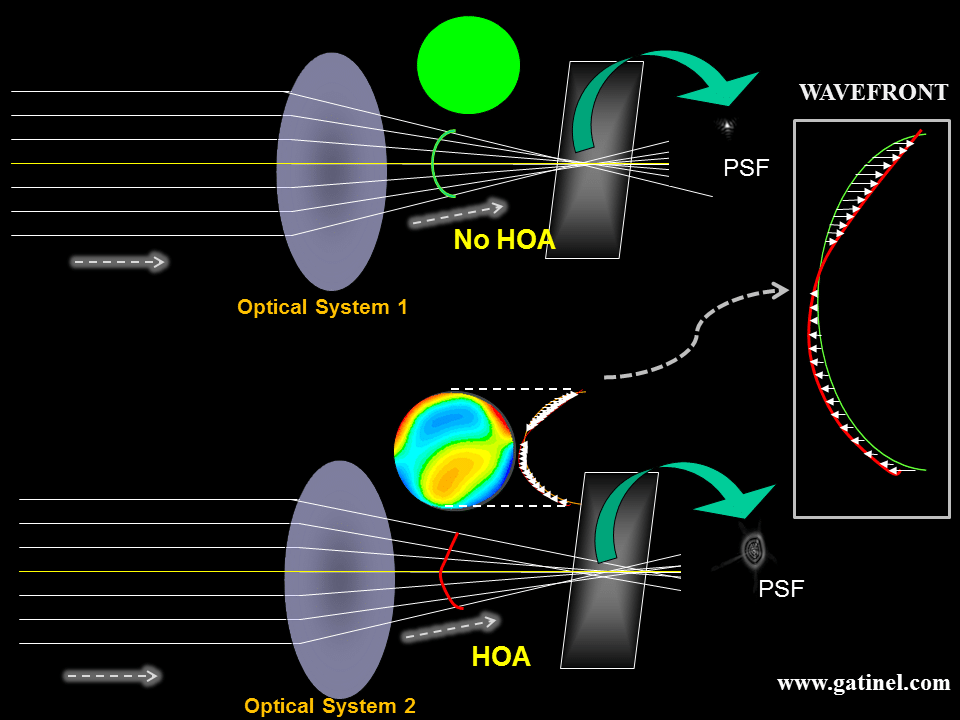
In geometrical optics, a perfect system brings all of the rays of an incident parallel bundle to the same focal point. When the system is free of optical aberrations, all the incident rays are refracted in a single focal point, which is called the « Point Spread Function (PSF) ». In the case of a non-aberrated system, the PSF is a point (of course, we have again ignored the effect of diffraction), and the surface of the refracted wavefront (in green) is a portion of a sphere ( or a circle in cross-section).Rays can be visualized as pointing in the direction of the propagation of the wavefront surface. In the case of a spherical wavefront, all the rays point toward the center of the sphere, and the center of that sphere coincides with the focal point.The spherical wavefront can serve as a « reference wavefront surface » since it embodies the wavefront formed by a perfect optical system. When incident light rays are not focused in the same location, due to optical aberrations, the refracted wavefront is no longer perfectly spherical. The differential between the shape of this aberrated wavefront and the «perfectly spherical » wavefront corresponds to the wavefront error.Aberrations can occur if the corneal curvature, the lens or intraocular lens position, and « optical powers » do not « match », ie, not all light waves interfere constructively at the same location. If light waves interfere at the same location, but if the retina is located in a different plane, this will result in pure defocus. Spectacles can selectively modify the optical path between central and peripheral rays to bring the constructive interference back to the foveal plane.In general, even when the best spectacle power is selected, human eyes will encounter imperfections which will alter the optical path along some rays (the optical path along the rays located at the periphery of the entrance pupil is slightly different to the optical path of the central rays). These imperfections correspond to what is known as « higher-order aberrations » in wavefront optics.
The Point Spread Function (PSF) and Strehl ratio
In the perfect eye, there are no differences in the optical path taken by each light wave leaving a very distant light source, and hitting the fovea, so all incoming light waves would interfere constructively at the fovea. However, even in a perfect eye, the law of physics prevents the light emitted by an even infinite light point source from forming a true image point – this is due to the phenomenon of diffraction (inherent to the wave property of light).
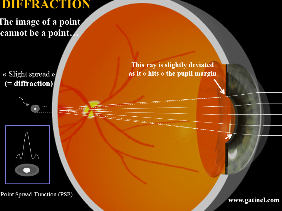
In a « perfect eye », also called a «diffraction–limited system », the point spread function (PSF) is not a point but a small bright disk (Airy Disk) surrounded by a very faint halo of light energy. Interestingly, the smaller achievable dimension of the central disk (1.5 microns) is about the same size of the smallest foveal cones (the effect of the pupil diffraction is minimized when the pupil is dilated). The measurement of the wavefront error enables to compute of the PSF using Fourier transform-based methods.
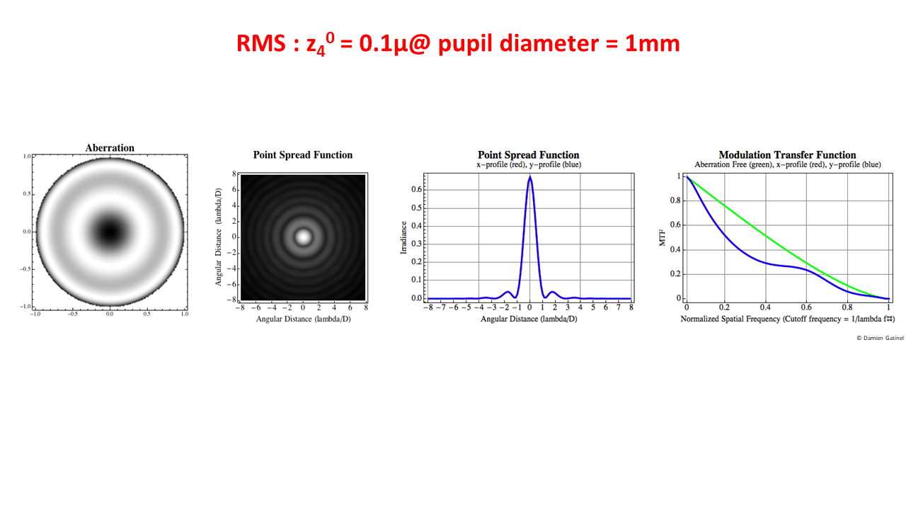
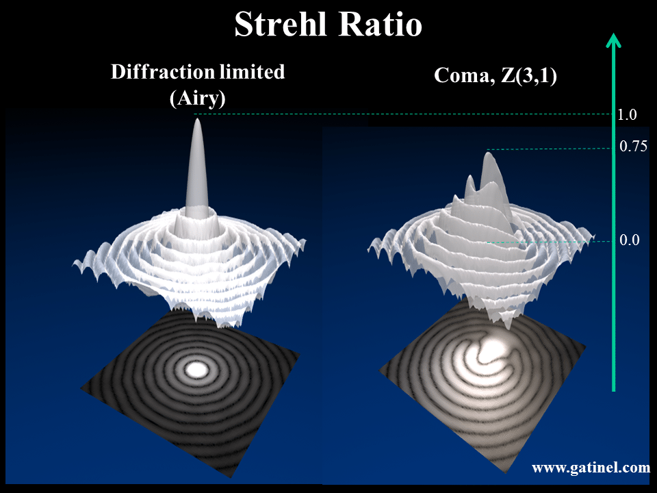
Contrast is plotted against spatial frequency (the level of resolution of the object image compared to the actual object being observed), with an MTF of 1 being the highest. )You can use this optic simulator to familiarize with the impact of specific or grouped aberrations. For a specific pupil diameter, the height of the peak of the diffraction-limited PSF can serve as a reference. The « Strehl ratio » corresponds to the ratio between the maximal height of the eye’s PSF and the diffraction-limited PSF. Because of the effect of the monochromatic aberrations which impair the optical quality of any biological system, such as the human eye, the monochromatic Strehl ratio of the « best » (least aberrated) eyes is usually not higher than 0.15.
What are the types of Aberrometers?
- Shack – Hartmann – Objective, Parallel, Double pass, Backward projection (eg. Zywave, WASCA, Multispot)
- Tscherning – Objective and subjective, Parallel, Double pass, Forward projection (Allegretto)
- Ray Tracing – Objective and subjective, Serial, Double pass, Forward projection (Tracey VFA)
- Automatic retinoscope – Objective, Serial, Double pass (Nidek OPD)
This section will focus on the basics of wavefront sensing and reconstruction as performed by an aberrometer.
The most commonly used wavefront analysis method is based on the Shack-Hartmann wavefront sensor, which was first used in the human eye in 1994. This method has quickly gained acceptance and popularity in the ophthalmic industry. Several commercial Shack-Hartmann eye aberrometers (ex, Zywave, Wavescan) offer acceptable measurement accuracy and reproducibility. For some highly aberrated eyes (keratoconus, post-complicated LASIK or PRK, post corneal transplant, post IOL dislocation) automated retinoscopy (OPDscan) or retinal ray tracing (iTrace) offers a better dynamic range than Shack-Hartmann instruments.
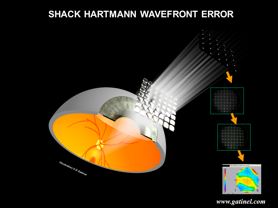
Schack-Hartmann wavefront sensing
After a bundle of infrared light, emitted by a laser diode, is focused at the foveal plane, its reflection forms an exiting wavefront which leaves the ‘entrance’ pupil of the eye, before being detected by a matrix of microlenses (lens array). The wavefront is sampled into small portions, each of which is focused on a CCD (Charged Coupled Device) sensor. The wavefront shape can be deduced from the location of the centroids (geometric center) of the spots array collected by the CCD sensor.
For example, in the case of a myopic eye, the collected wavefront will exhibit a spherical shape, which would collapse at the far point of the eye:
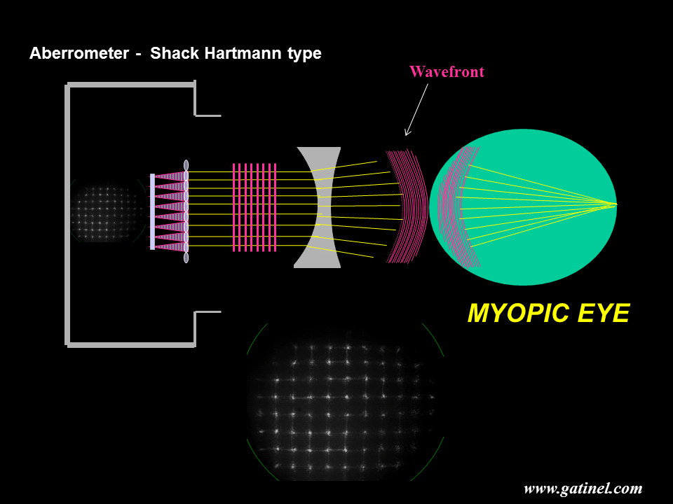
The wavefront shape of a myopic eye is dominated by spherical curvature, whose central radius is equal to the far point of the eye, where most of the wavefront collapses (if myopia is the only aberration of the measured eye, the wavefront entirely collapses at the far point). The Zernike defocus term also has a strong curvature. It is parabolic (a parabola is a curve obtained by plotting Y=X2,) and although the shape is not exactly spherical, the discrepancy can be discounted at that scale.When the exiting wavefront meets the surface of a “concave lens” with appropriate power (due to the curvature and refractive index >1 of the lens), its propagation speed decreases (inside the lens material – the wavelength shortens). Since the peripheral portion of the exiting wavefront reaches the lens medium before its center, the latter, which still travels in the air, gains some phase advance. This causes the wavefront to take on a flat geometry if the thickness of the concave lens is adjusted to cancel the phase shifts. The refraction of a purely flat wavefront forms a regular spot array after refraction by the micro-lenslet array of the Shack-Hartmann sensor. The power of the “concave lens,” which is required to flatten the wavefront, corresponds to the myopic error in that plane. If the wavefront is not perfectly flat, due to what is called “higher order aberrations”, the spot array is slightly irregular.
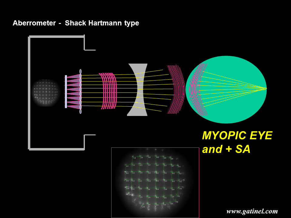
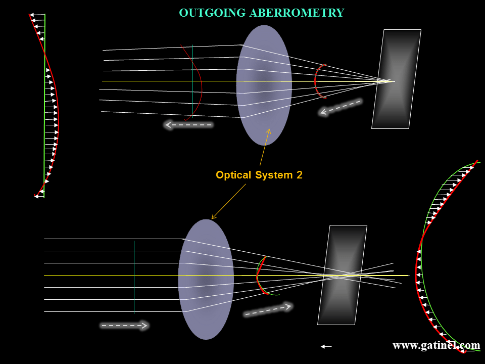
The shape of the wavefront can be measured from the departure of each spot from its expected position, that is, the position that the spot would occupy in the case of a purely flat wavefront (see next). Depending on the asphericity and refractive index of the lens, the wavefront may take on a spherical curvature and converge to a sharp focal point (no spherical aberration). Positive spherical aberration is caused when there is excessive bending of the wavefront periphery; due to this optical path difference, the peripheral rays may not interfere in phase with the central ones at the lens focal plane.Outgoing vs incoming aberrometry: It is important to note that wavefront aberrations of the human eye were usually measured using outgoing aberrometry, i.e, for a wavefront leaving the eye. In these situations, the reference wavefront is not a portion of a sphere, but a flat disc.
How is the Wavefront Analysed?
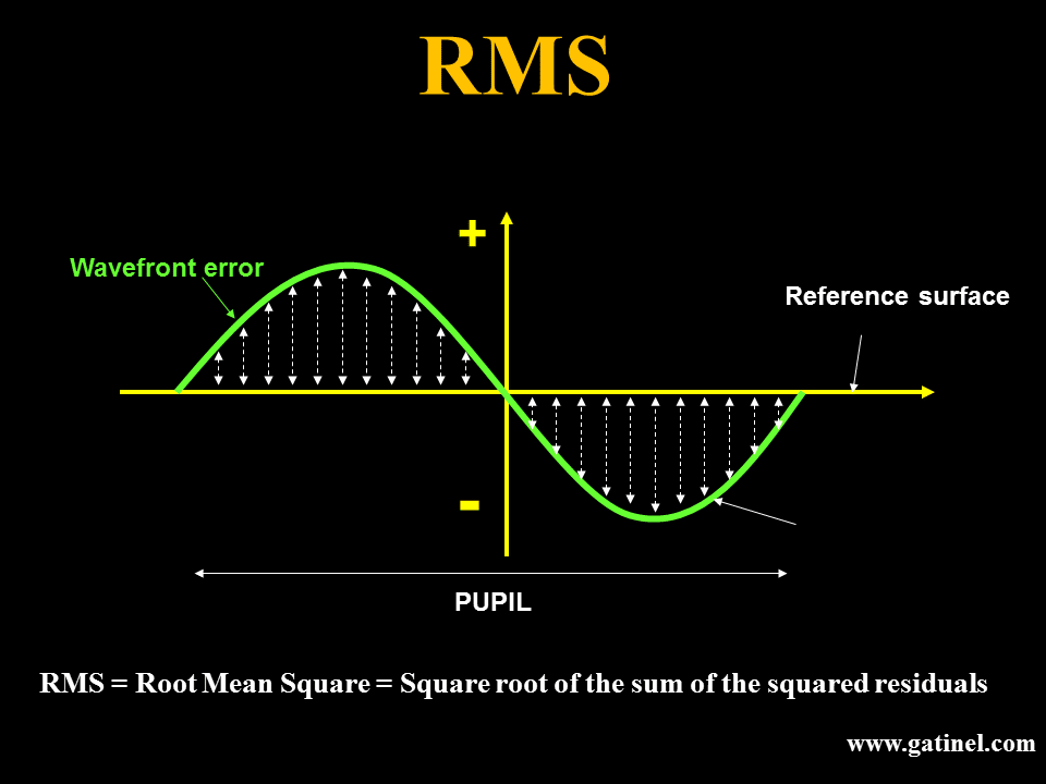
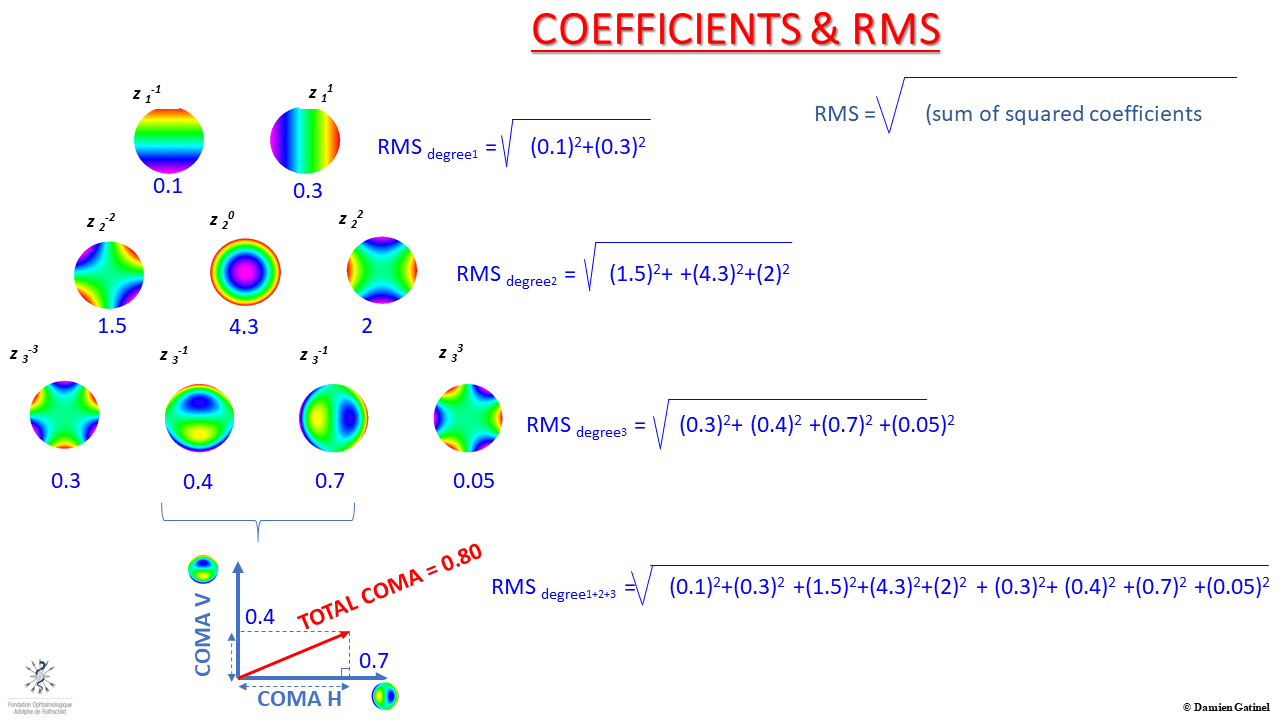
To analyse aberrations, the wavefront needs to be split into several components and adjusted by several mathematical equations. A few options included – Taylor series, Fourier analysis, and the commonest were Zernike polynomials.Currently, standardised (with American National Standards Institute ANSI) Zernike polynomial decompositions exist (standard double-index scheme), used specifically for optical wavefront aberration analysis. The Zernike polynomials are mathematical functions that are used to analyse and describe the wavefront error of the human eye. Some of the Zernike polynomials carry the name of classic optical aberrations: defocus, astigmatism, coma, trefoil… This terminology is also used by wavefront sensing instruments in their output.In addition, other optical quality metrics are usually associated with Zernike wavefront decomposition: Zernike coefficients, RMS, Strehl ratio, etc.Zernike polynomials are useful to express the wavefront error, which is a departure from the flat disk, as a sum of elementary deformations, which add up to reconstruct that wavefront error. It is useful to keep in mind that the latter corresponds to a variation from the expected optical path of the reference wavefront. It is generally expressed in ocular wavefront analysis as a distance unit, which is close to the dimensions of light waves: in microns(1 micron is 1/1000 of a millimeter). If you could measure the length of each arrow, take its square value, sum up all those squared values, and then take the square root of that total number, you would get the total RMS (Root Mean Square) value of the wavefront error. The RMS enables us to quantify the extent of the wavefront error.
Retina and Pupil Plane Metrics Uncovered
Visual performance metrics (relating ocular aberrations to visual performance) can be objective or subjective (neural input). In Objective metrics, we have talked about retina plane metrics (including Strehl and MTF) as well as the RMS value, which is a pupil plane metric. The RMS coefficient is an important concept. It allows quantifying the level of each of the aberrations that are involved in the wavefront error. An RMS coefficient refers to « one » single aberration mode (a Zernike mode), or a group of Zernike modes (eg, coma-like aberration RMS, which will include all 3rd degree aberrations).When the RMS of a group of aberrations has to be calculated, it is not achieved by adding the values of each RMS coefficient. Rather, each RMS coefficient is squared. The sum of these squared coefficients is then calculated. Finally, the global RMS is equal to the square root of the sum of the squared coefficients (reminiscent of Pythagoras’ Theorem a2+b2 = c2; the square of the hypotenuse is equal to the sum of the squares of the other two sides). These calculations are possible because the Zernike polynomials are orthogonal (perpendicular and discrete). Although orthogonality first evokes a particular spatial relationship between two lines or vectors, it can also be defined as a property of some analytical functions. The value of the RMS coefficient is very sensitive to the value of the wavefront domain diameter (pupil diameter).
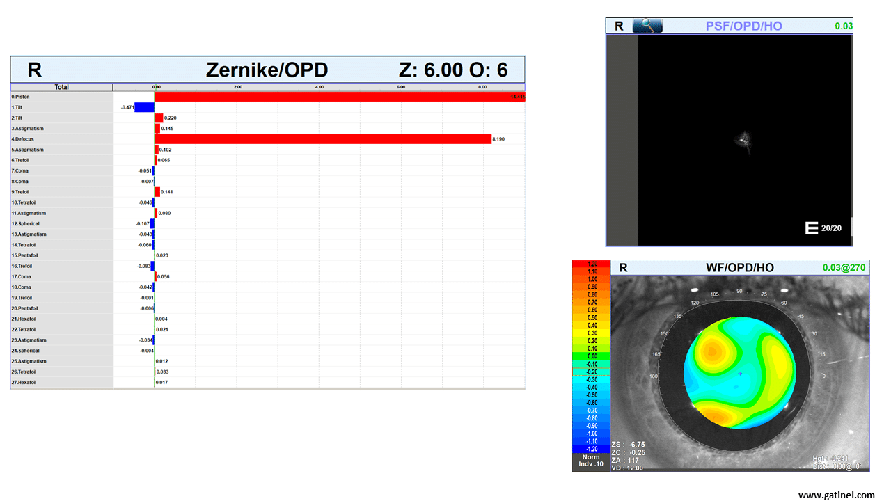
We hope now you can look at the wavefront analysis map below confidently, knowing what all the metrics and maps represent. It is important to note that in the real world, even ‘super-normal’ eyes have higher-order aberrations, and removing them doesn’t always translate to better functional vision. Retinal image degradation is affected by the composition of a stimulus, the type of aberration, and its interaction with other aberrations, with our neural input resulting in our visual perception.
We now have enough information to focus on the Zernike polynomials and their role in wavefront analysis.