Zernike polynomials
The Zernike polynomials
This page will focus on the use of Zernike polynomials for describing optical wavefronts. Before focusing on the Zernike polynomials, it is important to understand the basics of wavefront sensing.
Investigate the impact of Zernike aberrations on the quality of the retinal image
In ophthalmology and visual sciences, Zernike polynomials are mainly used to analyse the wavefront error of the human eye. It is also sometimes used to describe the shape of the cornea. The optical impact of the Zernike aberration modes can be visualised here.
Although the shape of the cornea dictates most of its optical properties, the Zernike polynomials cannot be interpreted interchangeably when they relate to the shape of an optical wavefront versus the shape of an optical surface.
Basically, Zernike polynomials can fit any surface defined on a circular domain.
The Zernike polynomials correspond to a kind of « taxonomy » for the optical aberration components that explain a wavefront error.
A wavefront error can be plotted with a color scale (micron step or wavelength units), on a domain that is the exit pupil disk.
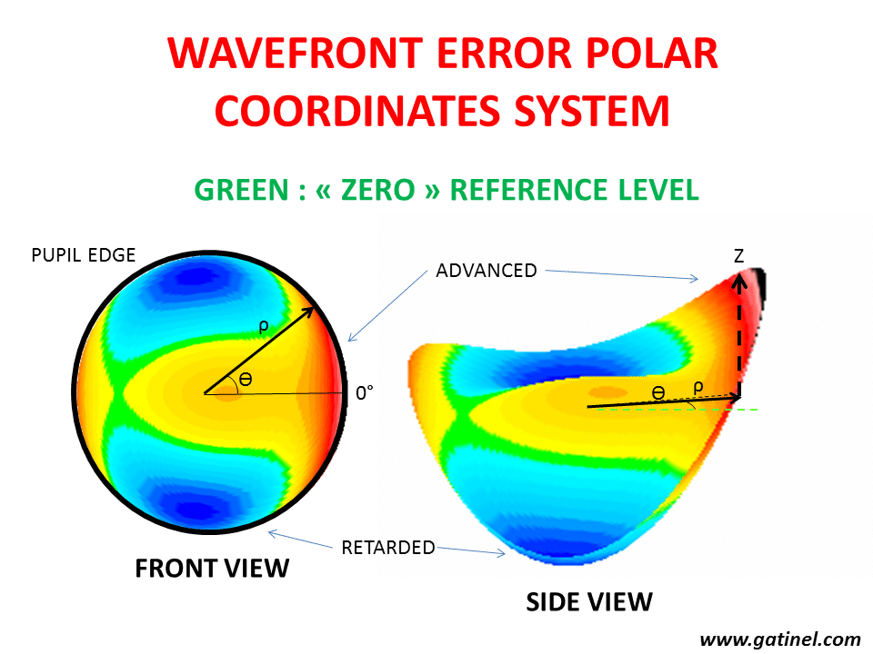
In the ANSI recommended polar coordinates system representation (2D system where the distance and angle of any point on the plane is calculated from the reference point and direction), the wavefront error depicts the optical path difference OPD (in microns) from the reference surface. The above representation corresponds to the OPD with a flat wavefront (green level). Each color step represents a phase shift of 1 micron. The zero level is the « mean » of the wavefront, which is the horizontal plane that separates into two equal components – the relatively advanced and delayed phases. The « height » of that zero level mean with regards to the lowest point of the wavefront error, corresponds to the RMS value of the first Zernike term, named piston (Z00).
NB: Zernike polynomials have some limitations in ophthalmic applications: they fail to segregate between low and higher-order aberrations. This reduces the clinical pertinence of the ocular wavefront decomposition in certain circumstances. We have proposed a new series of functions to overcome this limitation.
The Zernike pyramid
The Zernike modes are usually presented as a pyramid:
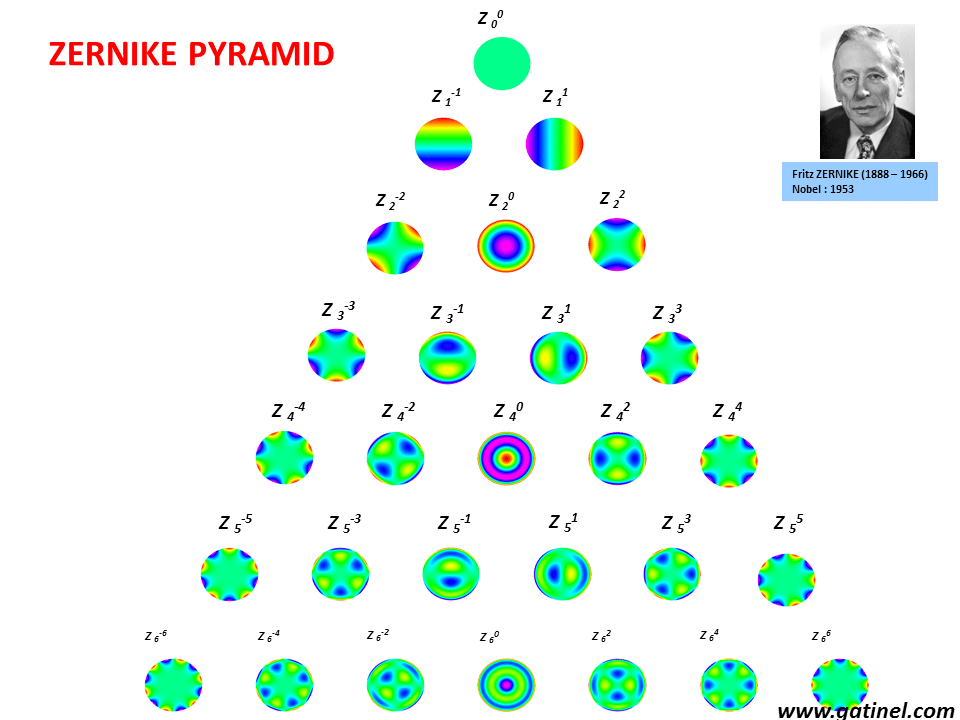
Representation of the Zernike pyramid formed by the first 28 modes (the Zernike pyramid has an infinite number of modes). The mean value of each mode (except for the piston) is zero. Think of each mode (or harmonic) as a kind of particular wavefront error within the pupil disk. Some modes, such as defocus (Z 20), are familiar to the clinician, whereas other (ex: tetrafoil : Z 4-4) are not.
If you are inclined to more abstract thinking, you can think of each mode as a unit vector. In a two-dimensional (2D) Cartesian domain, you could plot two unit vectors along the X and Y axes, which would be orthogonal (perpendicular and discrete) and with a Norm (function assigning positive length) equal to one.
In a 3D domain, you could add a third unit vector along the Z-axis, which is orthogonal to the X and Y axes. In such a 3D space, any vector can be decomposed into a weighted sum of the X, Y, and Z axis unit vectors.
In the « Zernike polynomial domain », you can extend such a concept to more than 3 « dimensions ». Each of these dimensions has its own unit vector, represented by a particular Zernike mode (each Zernike mode is normalized). Each of these dimensions would be perpendicular (orthogonal) to all the other ones.
In such a multi-dimensional space, a wavefront error would correspond to a particular vector, which could be « broken down » into a sum of weighted unit vectors (i.e, Zernike mode). The weight of each mode corresponds to the RMS coefficient of a Zernike wavefront decomposition. The orthogonality of the Zernike modes ensures that RMS computation is possible for a specified group of aberration modes.
You can try to relate the spatial shape of some Zernike modes to some ocular abnormalities:
1. Keratoconus: Characterized by some corneal vertical asymmetry, will easily induce vertical coma Z 3+/-1 (typically with a negative coefficient) in which the wavefront error is displayed vertically and introduce asymmetry between the superior and inferior half of the pupil domain. The coefficient of the coma term would be negative in most cases, as the wavefront error would show relative inferior delay (due to the inferiorly decentered apex) and a relative superior advance.
2. Radial Keratotomy: It may not be surprising to find high levels of trefoil Z 3+/-3 or tetrafoil Z 4+/-4 or any « higher-foils » Z n+/-n=m in eyes which have been operated with these techniques.
3. Pterygium: Horizontal coma Z 31 and trefoil Z 33 are frequently seen in advanced pterygia, due to the nasal corneal tear film distortion.
The Zernike polynomials analytical expression
The analytical expression of the Zernike polynomials may seem complex, and it is, but there are ways to break it down so that, as a clinician, you can understand its application.
Each Zernike mode, Znm is in fact a mathematical function with:
-
A normalizing constant (so that the square root of the sum of the squared residuals (errors) – RMS – of each function is equal to 1 on a pupil of radius = 1),
-
a polynomial in r,
-
for some modes, a trigonometric function of t is used.
-
n is a positive integer called the « radial degree » or « order »,
-
m is a negative or positive integer called the « azimuthal » or « angular frequency ».
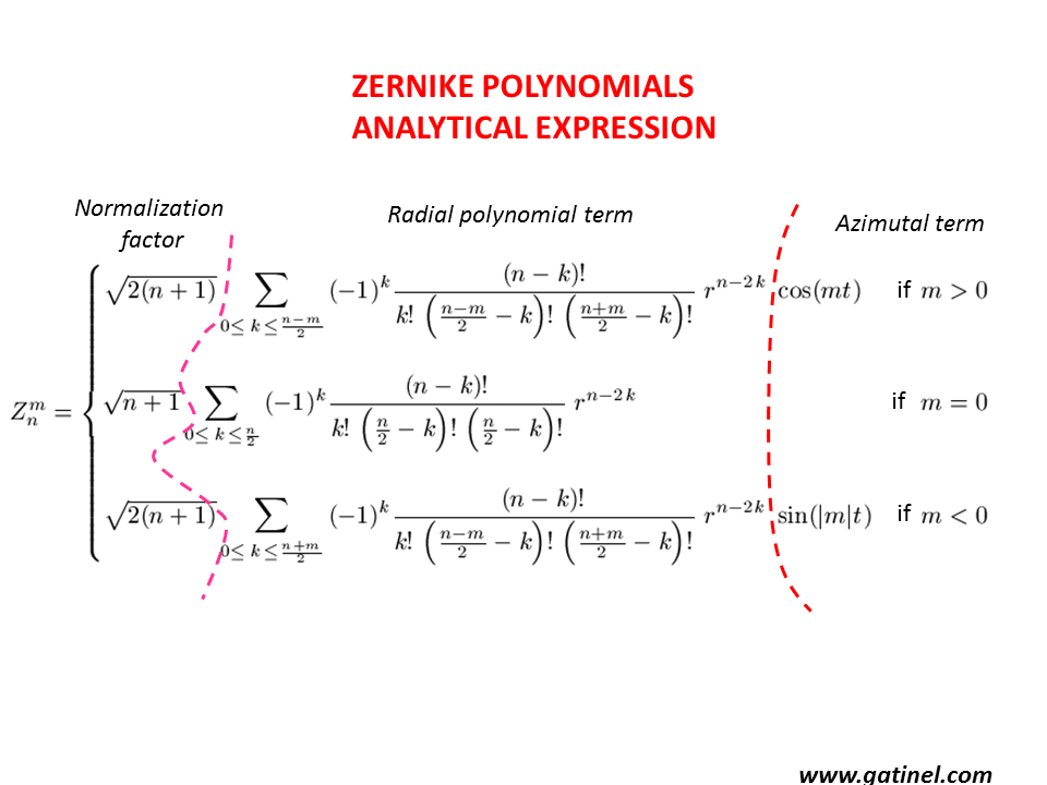
To obtain a particular Zernike mode of « n » radial degree and « m » azimuthal frequency, just insert the actual values of n and m in the equations. There is an important relation between n and m, which is conveyed by another variable « k », which is an integer comprised between zero and half of the sum or half of the difference between n and m. Because of these relations, the difference between the absolute values of n and m cannot be 1 or any odd number. Hence, there are no Z 10 or Z 4-3 Zernike polynomials. When m = 0, there is no angular dependence and the mode is « rotationally symmetrical,» eg, Defocus and Spherical aberration. Of course, regular astigmatism is azimuthally variable (m=2). The normalization factor is relatively straightforward to calculate; it just depends on n. It is a scaling factor, which makes the RMS of each mode equal to one on the unit pupil (radius = 1). It is important to note that the radial polynomial component can be constituted of the sum of terms of various radial degrees. Not all the Zernike modes are « pure » in their radial degree (more on this in our newly published paper).
n corresponds to the « degree » of a given mode. When n ≤ 2, the mode is said to be of a « lower » degree or LOA (Lower order aberrations).
Conversely, modes in which n ≥ 3 are said to be of a « higher » degree or HOA (Higher order aberrations).
Classically, spectacle corrected aberrations (myopia, hyperopia, and astigmatism) correspond to Zernike polynomials of radial degree n=2.
Let us focus on a Zernike mode named trefoil: Z 3-3. It may help the reader to connect the equation with the shape of the mode mentally.
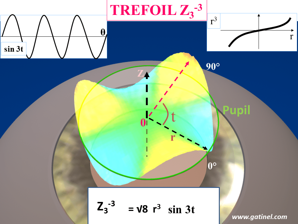
Representation of triangular astigmatism (trefoil) with the Z 3-3 polynomial on the normalized unit pupil disk (green ring). The surface of this mode is equal to the product of a 3rd order polynomial radial term (r3) where r is the radial distance from the pupil center, and a trigonometric function with an azimuthal frequency of 3 (sin3t), where t corresponds to the angle formed with the horizontal line (as for the common astigmatism axis angle plot). A normalization factor is a scaling number that makes each mode have a total RMS of unity. If you would like to visualize each mode as a vector, the normalization factor makes this vector a « unit vector », having a norm equal to one.
This is another Zernike mode called « secondary astigmatism« :
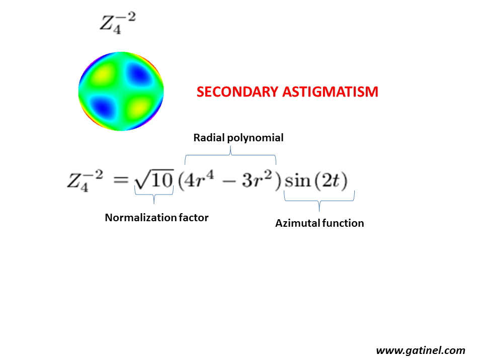
Example of a non-radially symmetrical Zernike mode (secondary astigmatism). This mode is formed by the product of a normalization factor, a radial polynomial (a function of r), and an azimuthal function (a function of t). Note that the radial polynomial is not « pure » in r4, but also contains lower-order azimuthal defocus (in r2). This explains the « tormented » shape of this mode. The presence of low-order terms in the radial polynomial of some high-order modes is due to the necessity of ensuring orthogonality with modes of lower radial degree but identical azimuthal frequency. It can cause artifacts in the low order wavefront coefficients.
The primary spherical aberration Z 40 is a « famous » Zernike mode:
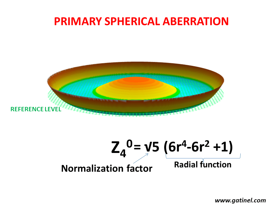
Example of a radially symmetrical Zernike mode (primary spherical astigmatism). This mode is formed by the product of a normalization factor, a radial polynomial (a function of r), but no azimuthal function; it is rotationally symmetrical. Note that the radial polynomial function is not « pure » in r4, but also contains lower order defocus (in r2)
The structure of the Zernike pyramid is based on the values of n and m:
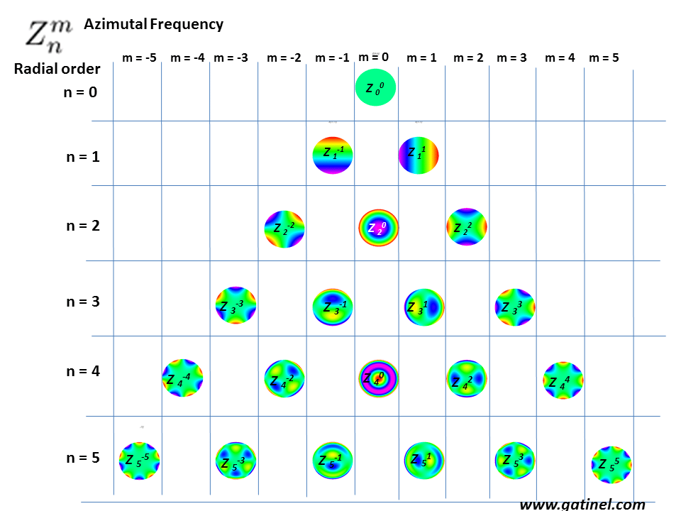
In the Zernike pyramid, the position of each polynomial depends on its radial order and azimuthal frequency.
In the central column, the modes are rotationally symmetrical (m=0), or unaffected by rotation. This central column can be seen as an axial symmetry axis.
On each line (same n value), the Zernike modes of opposite azimuthal frequency value have the same overall shape, but a different orientation.
These « pairs » are required to enable any mode resulting from the combination of the paired mode to be freely oriented around 360°. This is achieved by the respective weights (coefficients) of each mode of the pair to obtain the desired orientation.
For astigmatism, a purely « with a rule (WTR)» or « against the rule (ATR)» orientation would result in a null value of the « oblique » astigmatism component Z(2,-2) and some positive (ATR) or negative (WTR) RMS coefficient value of the Z(2,2) mode.
The first 6 Zernike polynomials correspond to « low order » aberrations (the highest radial term degree value is equal to 2). Spectacles can correct these aberrations.
From n=3 and beyond, the remaining modes correspond to « high order » aberrations. They cannot be fully corrected by spectacles.
However, contrary to popular belief, some modes such as spherical aberration (Z40) are containing some defocus (because of its term in r^2), and spectacles can correct this component. The remainder wavefront distortion in r^4, however, cannot. This may confuse some clinical situations.
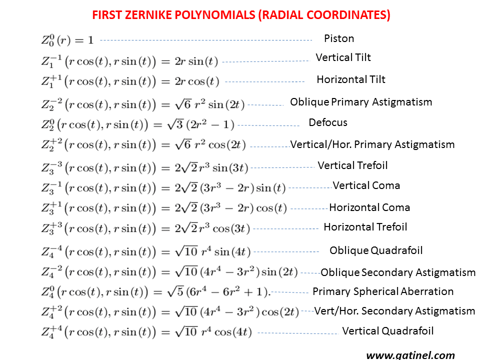
Here follows the analytical expression of the first Zernike modes in radial coordinates:
Sampling the wavefront error into Zernike modes
A wavefront error can be sampled, or decomposed, into Zernike modes; each RMS coefficient corresponds to the weight of the mode.
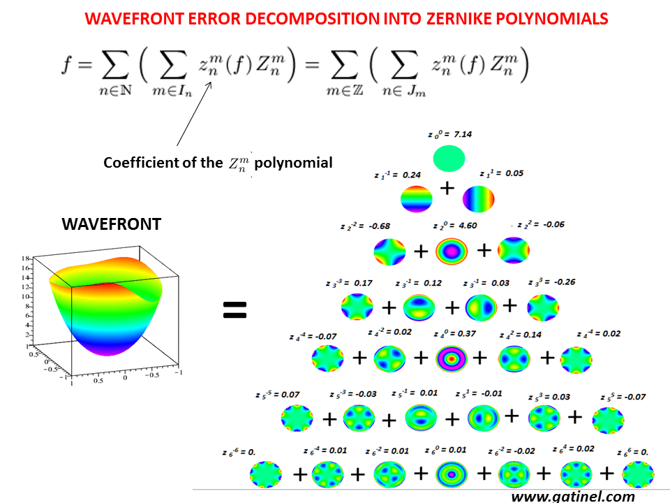
The total wavefront surface error (left) is equal to the sum of all the non zero RMS coefficients in the Zernike mode. The RMS value of this specific wavefront error is equal to the square root of the sum of all the squared coefficients.
The values of the coefficients are the direct consequence of the « shape » of the wavefront and of the diameter of the domain where it is measured. The larger the pupil diameter, the higher the absolute values of the Zernike coefficients. This increase is exponential; therefore, the higher the radial degree, the larger the amplitude of the variation with the pupil diameter.
Example:
This is an example of a wavefront reconstruction obtained with the wavefront sensor OPDscan III (Nidek)
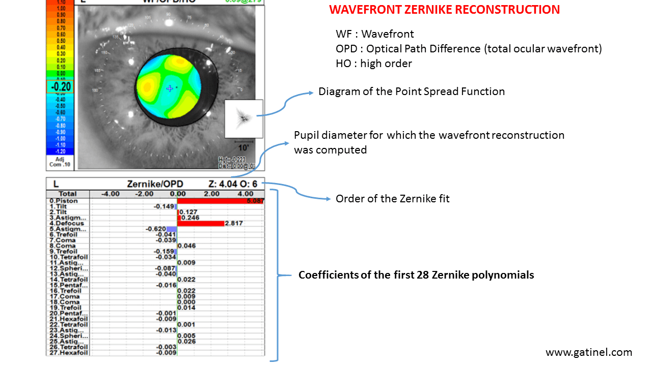
The wavefront sensor acquires optical data using a slit-scanning automated retinoscopy
See other relevant examples and material :
Novel wavefront decomposition method
Pre and Post LASIK aberrations